INTRO DOSE-RESPONSE

Figure 1. Laboratory test tubes for tox estimation by dose-response curves.
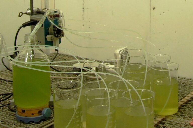
Figure 2. Growth cabinet test beakers for tox estimation by dose-response curves.
Dose-response curves are used to assess the toxicity of compounds in the laboratory, in growth chambers, and in the field. Whatever the environment, the principles are the same. An array of doses covers the effect from virtually no effect at low doses to high effect or the demise of a test organism at large doses.
There are constantly being evolved new methods to estimate toxicity. The use of dose-response experiments with living organisms, e.g., rats, mice, and guinea pigs, to assess the toxicity of compounds is being substituted with surrogate organisms or part of organs or isolated enzymes. With plants, we are more relaxed.
It isn’t easy to estimate the effects of a substance without testing it on living organisms. The chemical and physical properties of molecules tell us about their properties, but living organisms may react in unpredictable ways.
The bottom line is we use biological assays or in short bioassays to estimate the toxicological effects.
Bioassays are almost always with nonlinear dose-response-curves.

Figure 3. Dose-response experiment in the field. The individual strips are different herbicides affecting a test plant (canola).
A bioassay curve could look like this:
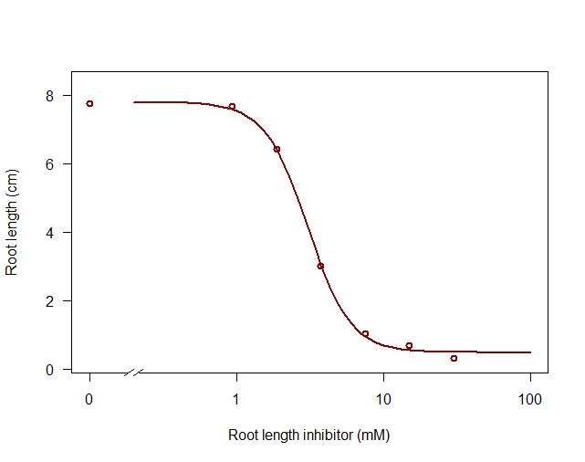
Figure 4. A dose-response curve with four parameters, the upper limit at zero dose and the lower limit at infinite large doses. A general estimate of the toxicity of a compound is the ED50. The fourth parameter is the relative slope at the inflection point, which for the log-logistic model coincides with ED50.
Bioassays are based on dose-response regressions from controlled experiments where a limited number of doses of a biologically active chemical are to be compared to a control group (dose 0).
Dose-response curves crystallize into a certain type of regression analysis of which the sigmoid curves, like the one in Figure 4, are very common.
Probit analysis is a specialized form of regression analysis applied to binomial response variables, i.e., variables with only one of two possible outcomes (positive/negative). The procedure transforms a dose-response curve into a straight line that facilitates a linear regression model. The estimation in the so-called probit regression model played an important role in the past. The probit analysis was a linearization of a logistic dose-response curve for qualitative data (dead/alive) in response to the doses.
Now nonlinear estimation of sigmoid curves became available through add-ons and macros for a spreadsheet. General-purpose statistical software programs also include nonlinear estimation procedures/but without any specific focus on dose-response analysis.
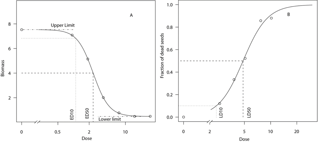
Figure 5. Graph A is a quantitative dose-response analysis where the y-axis may cover a range from – ∞ to infinity ∞. Graph B is the qualitative dose-response curve where the endpoint is the dead or alive seeds. Here the y-axis is limited between one and zero. In this particular instance, the upper and lower limit and the ED50 (Effective dose reducing the biomass halfway between the upper and lower limit) in A and LD50 ( Lethal dose where the upper limit of 1, e.g., all individuals dead and lower limit zero, e.g., no individuals dead). A has been analyzed with a 4 parameter log-logistic curve, B with a two-parameter curve. The relative slope around the EC50 or LD50 is the curves’ inflection point.
